Introduction to R
Department of Sociology | University of Texas at Austin
2026-01-22
Welcome to “Intro to R”
Course website (if you want to learn more):
- www.github.com/caseybreen/intro_r
- Slides, exercises, and solutions
Session goals
- Overview: why
Ris a powerful tool for social science research
- Introduction to
Rsyntax, data types, and data structures
- Basic understanding of data manipulation and visualization
Course agenda
- Module 1: Introduction to
R,RStudio,and code formats - Module 2:
Rprogramming fundamentals (syntax, operators, data types, data structures, sequencing) - Module 3: Working with data
- Module 4: Data manipulation and Visualization
Module 1
Introduction to R, RStudio, and code formats
Learning objectives:
Installing
RandRStudioWhy
R?Understanding
RScripts,Rnotebooks, Quarto documents
R and RStudio
Ris a statistical programming language- Download: https://cloud.r-project.org
RStudiois an integrated development environment (IDE) forRprogramming- Download: http://www.rstudio.com/download
Why R?
Free, open source — great for reproducibility and open science
Powerful language for data manipulation, statistical analysis, and publication-ready data visualizations
Excellent community, lots of free resources
Data visualization
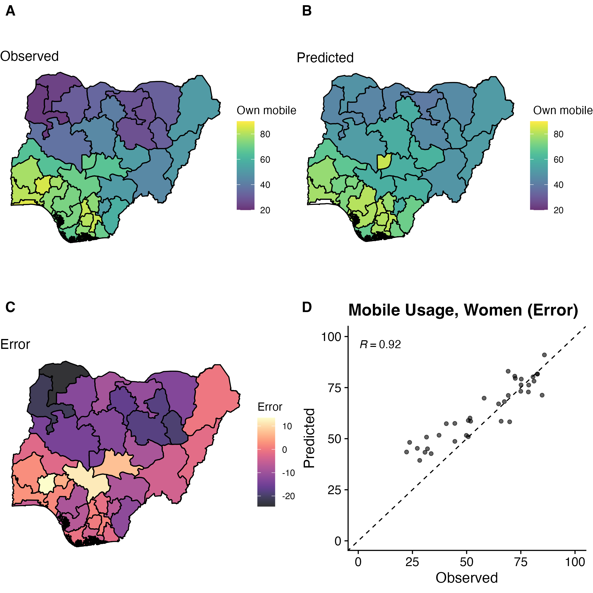
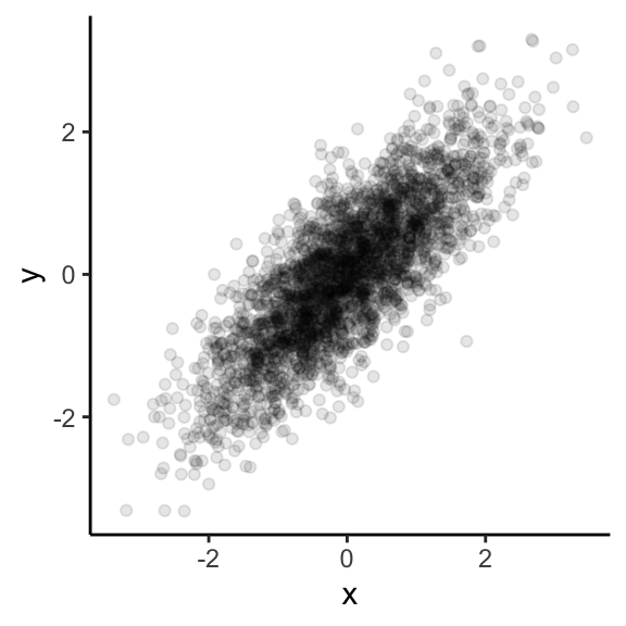
Easy to simulate + plot data
RStudio panes
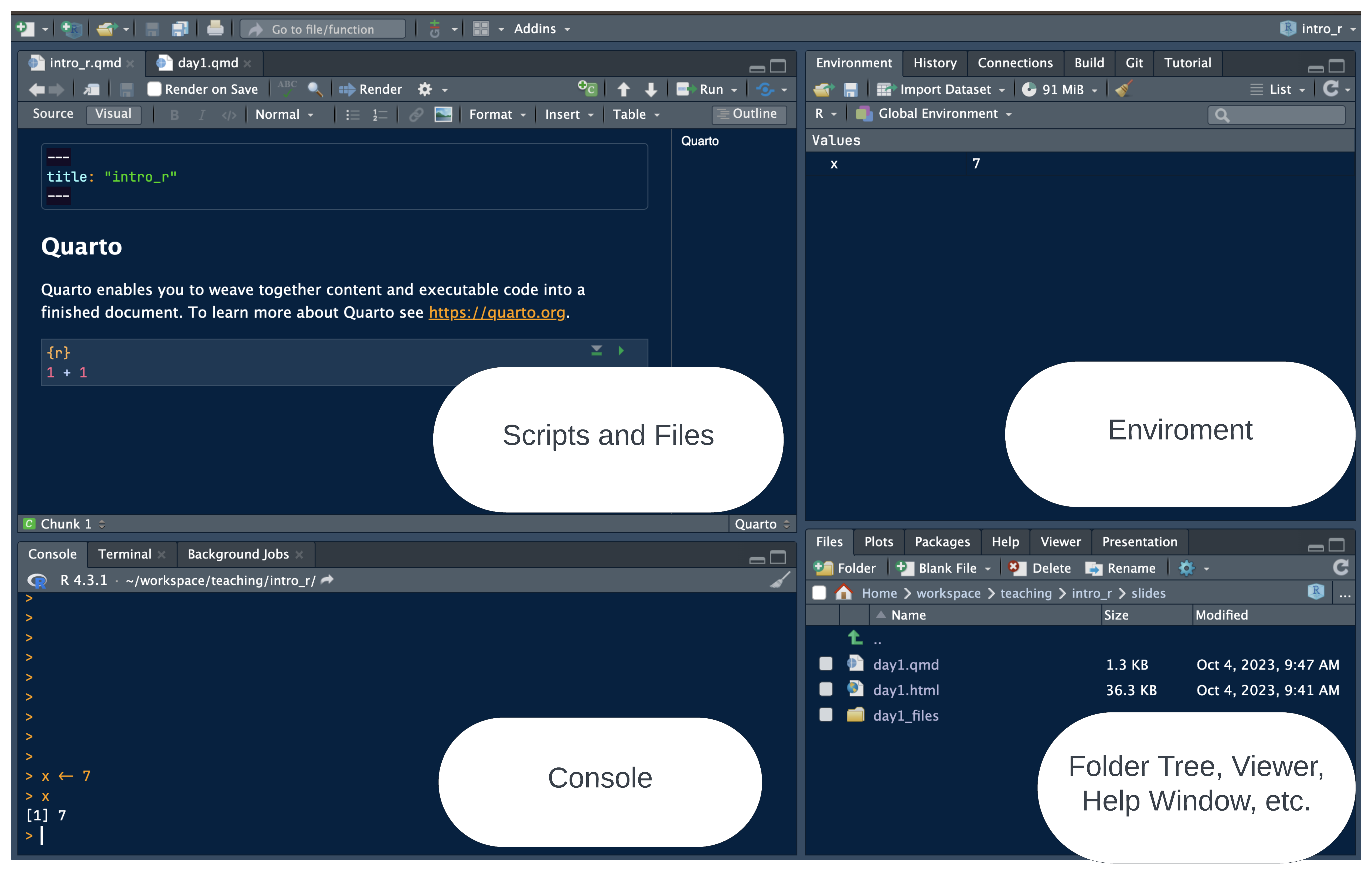
Why RStudio?
All-in-one development environment: streamlines coding, data visualization, and workflow
Extensible: supports R — but also Python, SQL, and Git
Rich community: eases learning and problem-solving
Code formats: R Scripts vs. R Notebooks
RScriptsSimple: just code
Best for simple tasks (and multi-script pipelines)
RNotebooks (Quarto,RNotebook)Integrated: Mix of code, text, and outputs for easy documentation
Interactive: real-time code execution and output display
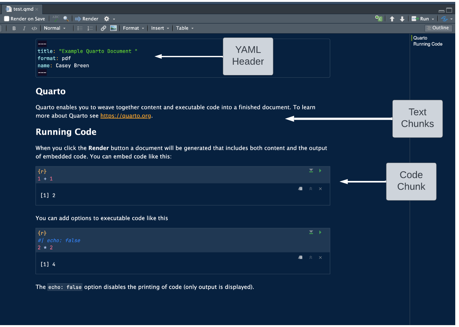
Quarto documents
“Notebook” Style: supports interactive code and text
Code cells: segments for code execution
Text chunks: annotations or explanations in Markdown format.
- Inline output: figures and code output display directly below the corresponding code cell
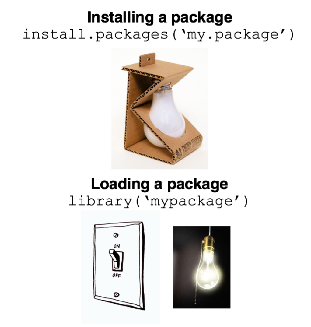
Installing packages
Running code
Run all code in a quarto document (or
Rscript, orRnotebook)- Exception: install packages, quick checks in console
To run a single line of code in a code cell
- Cursor over line,
Ctrl + Enter(Windows/Linux) orCmd + Enter(Mac).
- Cursor over line,
To run a full code cell (or script)
Ctrl + Shift + Enter(Windows/Linux) orCmd + Shift + Enter(Mac).
Live coding demo
- Demo of creating a new Quarto document and running code in a code cell
- Your turn next…
In-class exercise 0
Create a new quarto document
File -> New File -> Quarto Document -> Create
Create a new code cell
Insert -> Executable cell -> R
Practice running code below
Module 2
R programming fundamentals
Learning objectives:
Comprehend R objects and functions
Master basic syntax, including comments, assignment, and operators
Understand data structures and types in R
Objects
- Everything in R is an object
Vectors: Ordered collection of same type
Data Frames: Table of columns and rows
Function: Reusable code block
List: Ordered collection of objects
Functions
- Built-in “base” functions
- Custom, user-defined functions
[1] 7- Functions from packages
Assignment operators
Use
<-or=for assignment<-is preferred and advised for readability
Formally, assignment means “assign the result of the operation on the right to object on the left”
Arithmetic operators
- Addition / Subtraction
- Multiplication / division
- Exponents
Comparison and logical operators
Operators
| Operator | Symbol |
|---|---|
| AND | & |
| OR | | |
| NOT | ! |
| Equal | == |
| Not Equal | != |
| Greater/Less Than | > or < |
| Greater/Less Than or Equal | >= or <= |
| Element-wise In | %in% |
Data structures
There are lots of data structures; we’ll focus on
vectorsanddata frames.Vectors: One-dimensional arrays that hold elements of a single data type (e.g., all numeric or all character).Data frames: Two-dimensional tables where each column can have a different data type; essentially a list of vectors of equal length.
Vectors and data frames
Vectorexample
[1] 1 2 3 4 5Data frameexample
Data types
Each
vectorordata framecolumn can only contain one data type:Numeric: Used for numerical values like integers or decimals.Character: Holds text and alphanumeric characters.Logical: Represents binary values - TRUE or FALSE.Factor: Categorical data, either ordered or unordered, stored as levels.
NA (missing) values in R
NArepresents missing or undefined data.- Can vary by data type (e.g.,
NA_character_andNA_integer_)
- Can vary by data type (e.g.,
NAvalues can affect summary statistics and data visualization.What happens when you run the code below?
Generating sequences in R
- Method 1: Manually write out sequence using
c()
- Method 2: Colon operator (
:), creates sequences with increments of 1
- Method 3:
seq()Function: More flexible and allows you to specify thestart,end, andbyparameters.
Functions
Function: Input arguments, performs operations on them, and returns a result
For each of the below functions, what are the:
Input arguments?
Operations performed?
Results?
Keyboard shortcuts
Insert new code cell
macOS:
Cmd+Option+IWindows/Linux:
Ctrl+Alt+I
Run full code cell or script
macOS:
Cmd+Shift+EnterWindows/Linux:
Ctrl+Shift+enter
Assignment operator (creates <-)
macOS:
option+-Windows/Linux:
option+-
Live coding demo
Assignment (e.g.,
x <- 4)Logical expressions (e.g.,
x > 10)Creating a basic sequence
Your turn next…
In-class exercise 1
- Assign
xandyto take values 3 and 4. - Assign
zas the product ofxandy. - Write code to calculate the square of 3. Assign this to a variable
three_squared. - Write a logical expression to check if
three_squaredis greater than 10. - Write a logical expression testing whether
xis not greater than 10. Use thenegatesymbol (!).
Exercise 1 solutions
- Assign
xandyto take values 3 and 4.
- Assign
zas the product ofxandy.
- Calculate the square of 3 and assign it to a variable called
three_squared.
- Write a logical expression to check if
three_squaredis greater than 10.
- Write a logical expression to test whether
three_squaredis not greater than 10. Use thenegatesymbol (!).
Module 3
Working with vectors and data frames
Learning objectives
Select elements from
vectorsand columns fromdata framesSubset
data framesInvestigate characteristics of
data frames
Indexing vectors
- Basic indexing
[1] 1[1] 3- Conditional indexing
Working with data frames
Data framesare the most common and versatile data structure inRStructured as rows (observations) and columns (variables)
| id | name | age | gender | score |
|---|---|---|---|---|
| 1 | Alice | 25 | F | 90 |
| 2 | Bob | 30 | M | 85 |
| 3 | Carol | 22 | F | 88 |
| 4 | Dave | 28 | M | 92 |
| 5 | Emily | 24 | F | 89 |
Working with data frames
head()- looks at top rows of thedata frame$operator - access a column as avector
Subsetting data frames
Methods:
$: Single column by name.df[i, j]: Rowiand columnj.df[i:j, k:l]: Rowsitojand columnsktol.
Conditional Subsetting:
df[df$age > 25, ].
Quiz
Which rows and will this return?
- Which rows and which columns will this return?
Answers
Explore data frame characteristics
Check number of rows
Check number of columns
Check column names
Module 4
Data manipulation and visualization
Learning objectives
Overview of
tidyversesuite of packagesFundamentals of data manipulation with
dplyrData visualization with
ggplot
Tidyverse
- Packages: Collection of R packages designed for data science.
- Data manipulation: Simplifies data cleaning and transformation with
dplyr. - Data Visualization: Enables advanced plotting with
ggplot2.
Data Manipulation using dplyr
filter: Select rows based on conditions.
select: Choose specific columns
mutate: Add or modify columns
summarize or summarise: Aggregate or summarize data based on some criteria
group_by: Group data by variables. Often used with summarise().
The Pipe Operator %>% (or |> ) in R
Takes the output of one function and passes it as the first argument to another function
- “And then do…”
What’s the below code doing?
Recoding values in R
Sometime you want to recode a variable to take different values (e.g., recoding exact income to binary high/low income variable)
The
case_when()function inRis part of thedplyrpackage and is used for creating new variables based on multiple conditions:
Live coding demo
Filter data
Selecting data
Calculating summary statistics by group
Creating and recoding variables
Your turn
# A tibble: 6 × 10
  carat cut       color clarity depth table price     x     y     z
  <dbl> <ord>     <ord> <ord>   <dbl> <dbl> <int> <dbl> <dbl> <dbl>
1  0.23 Ideal     E     SI2      61.5    55   326  3.95  3.98  2.43
2  0.21 Premium   E     SI1      59.8    61   326  3.89  3.84  2.31
3  0.23 Good      E     VS1      56.9    65   327  4.05  4.07  2.31
4  0.29 Premium   I     VS2      62.4    58   334  4.2   4.23  2.63
5  0.31 Good      J     SI2      63.3    58   335  4.34  4.35  2.75
6  0.24 Very Good J     VVS2     62.8    57   336  3.94  3.96  2.48
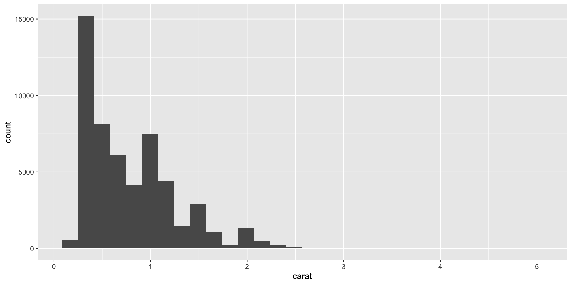
Data Visualization (Distn of carats)
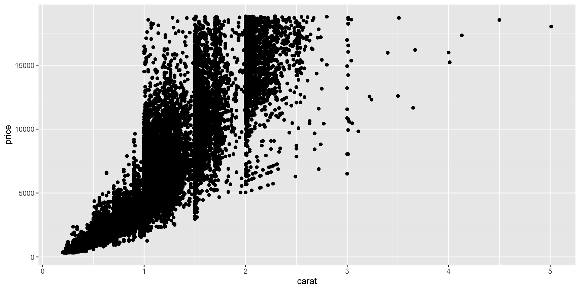
Data Visualization (Carat vs. Price)
Exercise
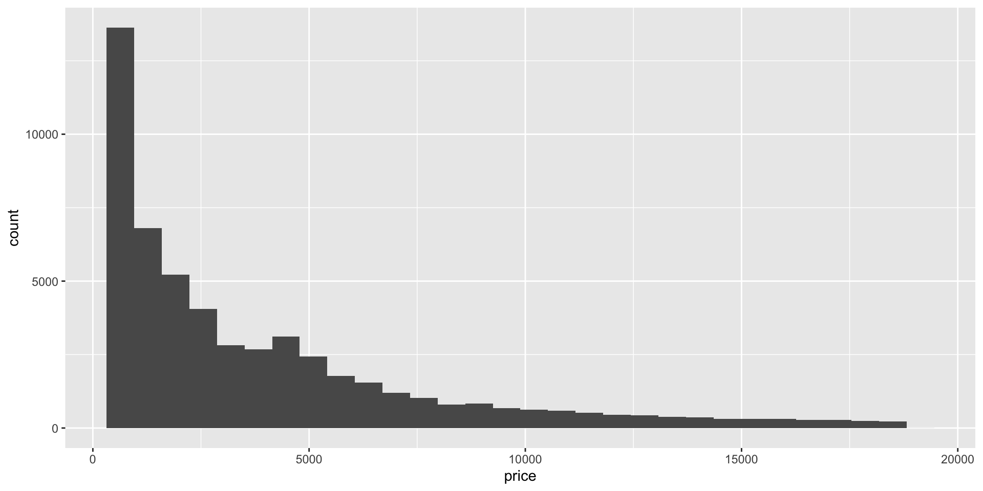
Make a histogram of the price of diamonds
For diamonds great than 1 carat (hint:
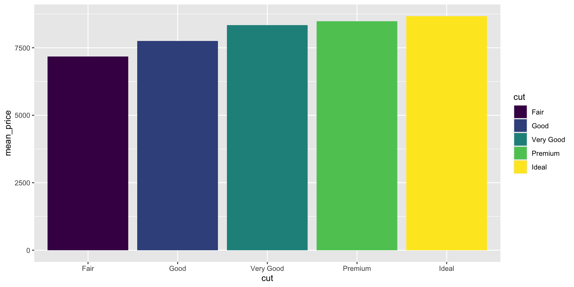
filter()), what is average price bycut(hint:group_by+summarize?Assign your answer from (2) to a data.frame called
price_by_cut. Now useggplot()+geom_colto visualize this.
Solutions Q1
Solutions Q2
Solutions Q3
Resources for learning more
R for data science (https://r4ds.hadley.nz/)
Data visualization: a practical introduction (https://socviz.co/)
Turn in your lab!
Please turn in your Qmd file (whatever you have completed) on Canvas so you can get credit.
Comments
Use
#to start a single-line commentComments are an important way to document code